---
title: "Discrete-Time Discrete-Loci Structured Wright Fisher Malaria Model Overview"
output: rmarkdown::html_vignette
vignette: >
%\VignetteIndexEntry{Discrete-Time Discrete-Loci Structured Wright Fisher Malaria Model Overview}
%\VignetteEncoding{UTF-8}
%\VignetteEngine{knitr::rmarkdown}
editor_options:
chunk_output_type: console
---
```{r, include = FALSE}
knitr::opts_chunk$set(
collapse = TRUE,
comment = "#>"
)
```
```{r setup}
library(polySimIBD)
```
# Purpose
The purpose of the `polySimIBD` package is to perform forwards in-time simulation of malaria population genetics. The model uses a discrete-time, discrete-loci structured Wright Fisher approximation to account for (simplified) malaria transmission dynamics.
# A Primer on Malaria Genetics
The need for a malaria-specific simulator is primarily due to the complex life-cycle of malaria and the phenomenon of multiple strains potentially infecting a single human host ("Complexity of Infection", or "Multiplicity of Infection"). As part of the malaria life-cycle, parasite ploidy switches from haploid in the human host to diploid in the mosquito vector midgut. It is during this diploid stage that recombination occurs between parasites. However, not all recombination results in unique progeny, or unique haplotypes. For example, if only a single haplotype is present in the mosquito midgut (i.e. a monoclonal infection), all recombination events will "look" the same, as there is no variation for recombination to act upon. In contrast, if more than one haplotype is present in the mosquito midgut (i.e. a polyclonal infection), recombination will produce unique progeny.
In a similar framework, hosts can then be infected with monoclonal or polyclonal infections depending on the number of infectious bites they receive and the number of unique haplotypes within the mosquito vector at the time of the infectious bite. As a result, host polyclonal infections can result either from:
1. Multiple infectious bites transferring unique haplotypes (Superinfection)
2. A single infectious bite transferring multiple haplotypes (Co-Transmission)
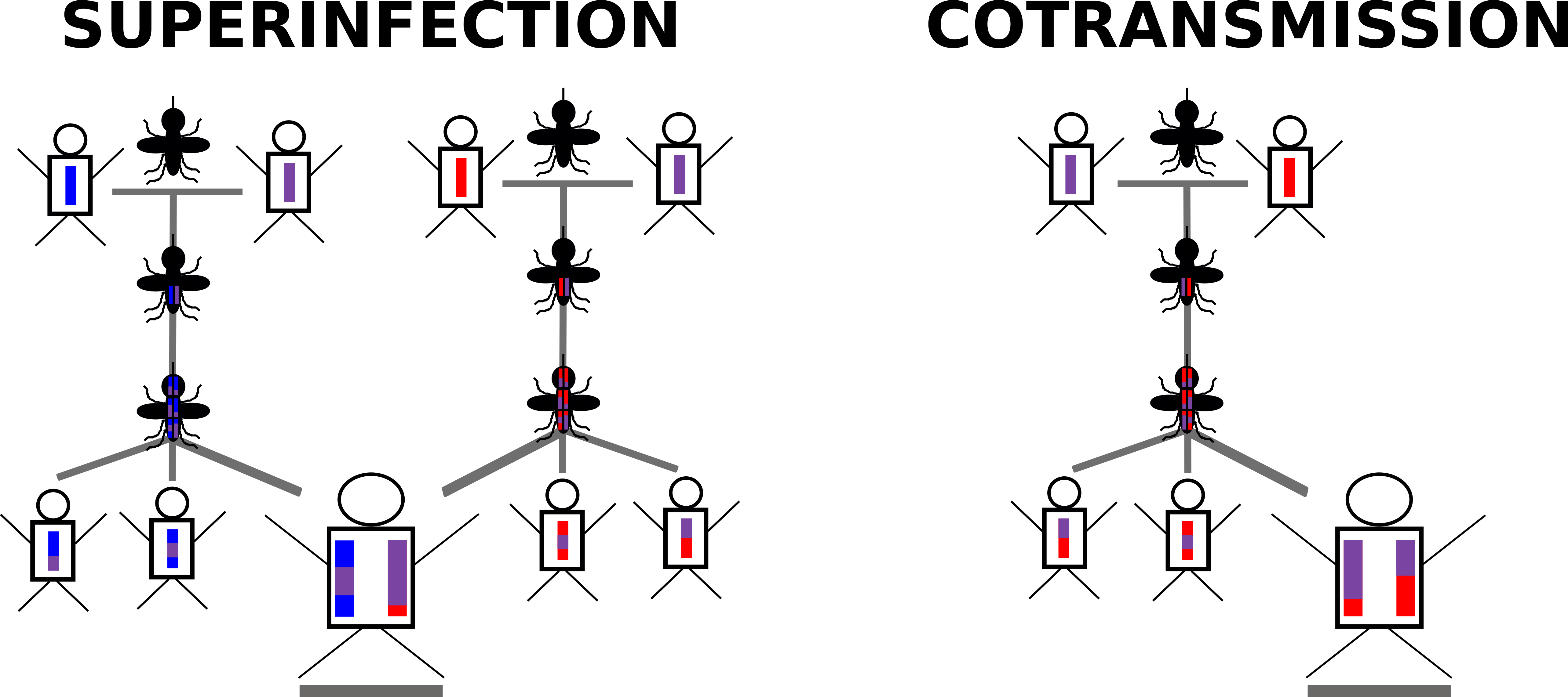{width=500px}
# A Primer on the Coalescent
Coalescent theory is one of the central pillars of population genetics and is a vast subject (see Wakeley's classic textbook, [Coalescent Theory: An Introduction](https://www.amazon.com/Coalescent-Theory-Introduction-John-Wakeley/dp/0974707759)). Essentially, the coalescent theory provides a framework for how loci (genes, individuals, etc.) have been derived from a common ancestor backwards in time, classically using the assumptions of the Wright-Fisher model. One of the main assumptions of the coalescence, is that loci are independent and that no recombination is occurring between loci. To relax this assumption, we must consider the coalescence with recombination. In this framework, a single coalescent tree is no longer representative of the genome (_NB_: genomes are now combination of genes on intervals [0, L) ; [L, L_{+1}], see [Griffiths & Marjoram 1996](http://lamastex.org/recomb/ima.pdf) for further details). Thus, each recombination event creates a marginal tree, or an independent genealogical history, for the given interval. The collection of these trees is termed the Ancestral Recombination Graph (ARG).
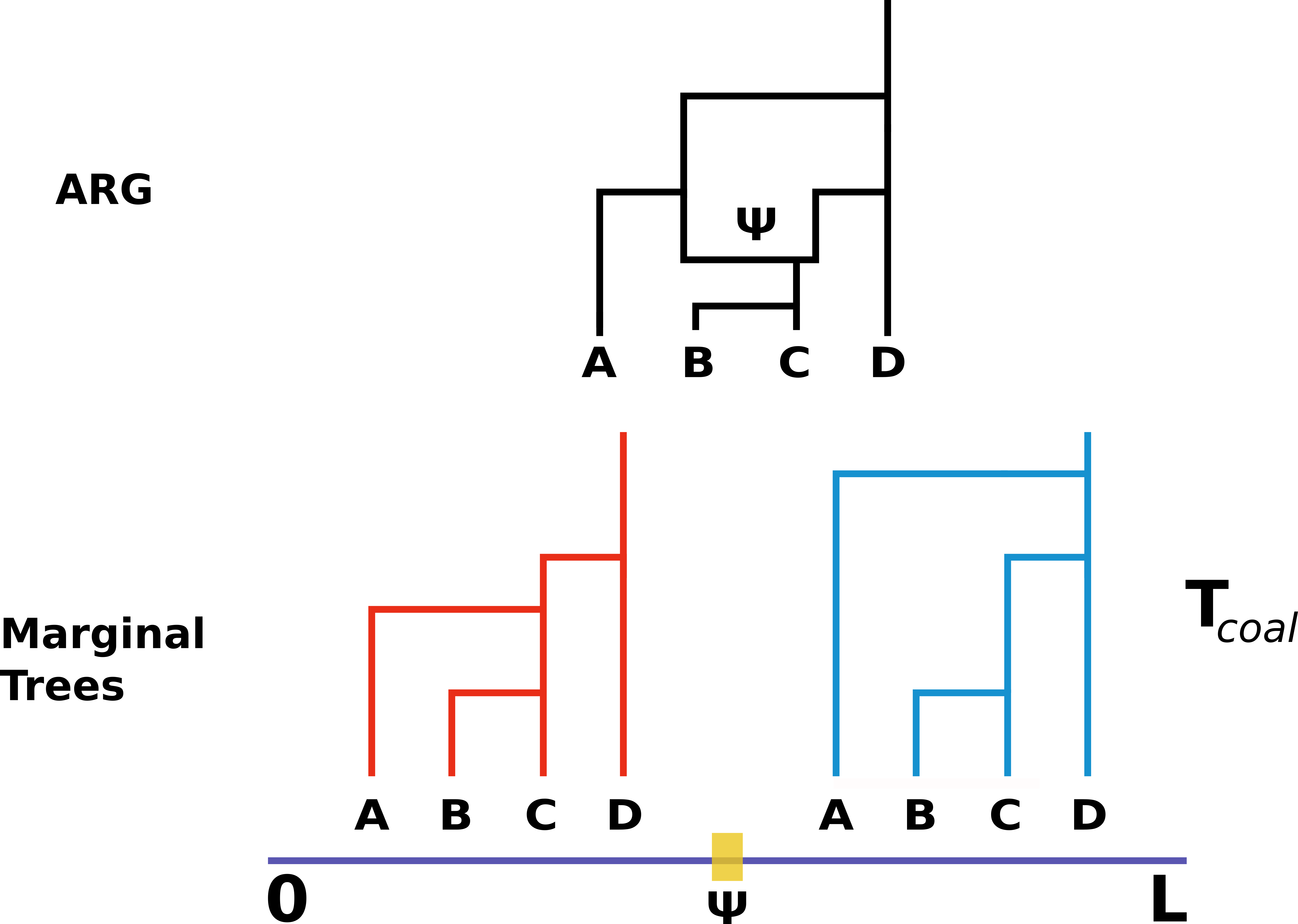{width=500px}
# Model Formulation
The full mathematical formulation of the (nonspatial) model can be found in the Supplementary Section of [Verity, Aydemic, Brazeau _et al._ Nat Comms 2020 (PMC7192906), Biorxiv](https://www.nature.com/articles/s41467-020-15779-8). In brief, we assume that each individual host can be represented by a deme, or a subpopulation within a large population ($i \in N$, where $i$ is an individual host and $N$ is the total host population). We then allow the $j$ parasites (that reside within the host population) to mate at random with the previous generation of parasites ($t_{1-}$) and produce a large number of parasite progeny. During mating, genetic recombination has the potential to occur based on the length of the genome and the recombination rate, $\rho$. Progeny are then allowed to migrate to a new or the same host with a probability of $\frac{m}{N}$. Finally, progeny are culled to a smaller number of parasites per host by drawing from a Poisson distribution with a mean COI (schematic below). This creates the new generation of parasites within hosts (i.e. infections). Overall, the simulator is best described as a discrete-loci, discrete-time structured Wright Fisher model.
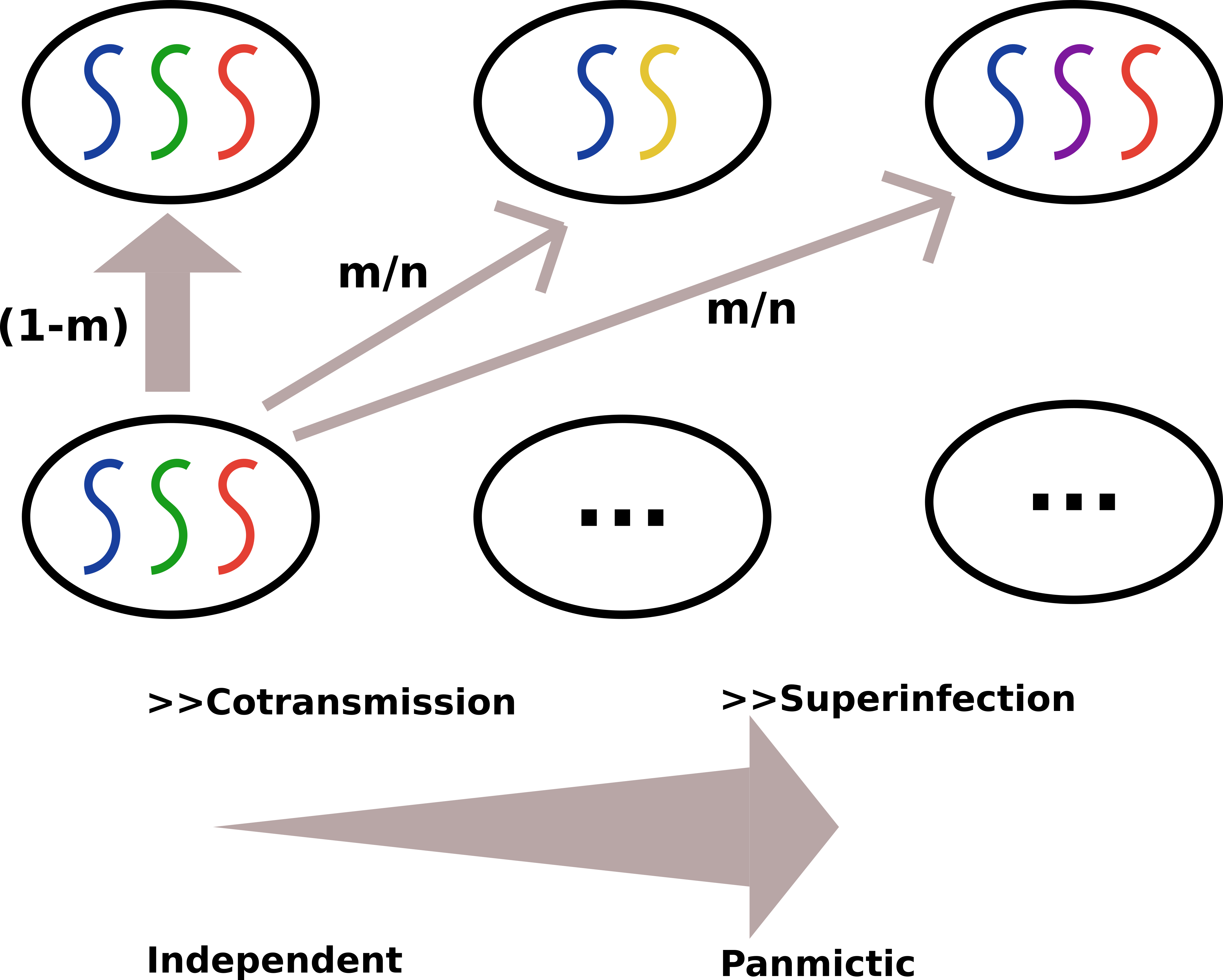{width=500px}
As can be seen from the schematic, the user-specified probability of migration, $m$, has an effect on whether or not the transmission dynamic favors Superinfection ("panmictic") or Contransmission ("independent") setting.
# Understanding the Simulator
Users are able to specify loci positions, `pos`, the number of hosts in the population, `N`, the probability of migration, `m`, the recombination rate, `rho`, and the mean COI, `mean_coi` (i.e. the host parasite burden and culling of the progeny). Finally, users have the option to let the model run forwards in time until all parasites have coalesced to a single common ancestor (`tlim = Inf`), or can set a limit on the number of generations that we simulate (`tlim = `).
```{r}
set.seed(1)
swfsim <- sim_swf(pos = seq(1, 1e3, 1e2),
N = 5,
m = 0.5,
rho = 1e-3,
mean_coi = 2,
migr_mat = 1, # nonspatial
tlim = 10)
```
The discrete-time, discrete-loci structured Wright Fisher simulation outputs six objets:
1. A vector of COIs, where each item in the vector is the number of parasites within a given host
2. A list of recombination blocks for each generation for each haplotype
3. The host and haplotype within the host parental assignments, respectively (i.e. identifiers for the "maternal" host and "maternal" haplotype and vis-versa for "paternal" identifiers for each progeny).
}
The output of this function is largely for internal use and is intended to be parsed and summarized with the `get_arg` function (next section).
# Getting the ARG
From the simulation above, we can derive the most recent common ancestor (MRCA) and the time of coalescence for each parasite (i.e. haplotype) at each discrete loci. In other words, we are recreating a marginal tree for each loci and then collectively storing the entire set of marginal trees, termed the ancestral recombination graph. _Note_, in our
simulation, loci may have identical marginal trees, as loci represent genetic markers
and not necessarily solely recombination events.
```{r}
ARG <- get_arg(swfsim, host_index = c(1,2))
```
The `get_arg` function takes the output from the discrete-loci, discrete-time structured Wright Fisher simulation above and produces a margianl tree: `bv_tree` for each loci.
### `bv_tree` Class
The `bv_tree` class is a lightweight representation of a marginal tree. The `bv_tree` class contains three slots:
1. `c`: The node connection for each haplotype (each haplotype is an element in a vector)
2. `t`: The timing of the node connection (time to MRCA)
3. `z`: The order of coalescence for each set of haplotypes
You may have noticed that our coalescent trees (`bvtree` class) always coalesce "right-to-left". This is intentional and an approach to optimize looping through ancestries to get the ARG.
# Tree Conversions
Separately, `polySimIBD` provides the functionality to convert a `bvtree` into a [Newick tree](https://en.wikipedia.org/wiki/Newick_format). This allows use to export results into other packages, such as[`ape`](https://cran.r-project.org/web/packages/ape/index.html). The conversion is limited to a single `bvtree` at a time, but this can easily be leveraged for the ARG with an iterative function. Note, you must manually re-enter the `tlim`, or the maximum number of generations considered in your simulation (i.e. the ARG
does not "remember" the tlim".
```{r, eval=FALSE}
bvtreeToNewick(bvtree = ARG[[1]], tlim = 10)
```
# Conclusion
Up until this point, we have ignored spatial considerations and migration of parasites between demes. In the next section, we will relax this assumption and analyze how space effects parasite genomic dynamics.